
Humans are great at classifying noises. We can hear a chirp and surmise that it belongs to a bird, we can hear an abstract noise and classify it as speech with a particular meaning and definition. This relationship between humans and audio classification forms the basis of speech and human communication as a whole.
This post was originally published in Dolby.io.
Translating this incredible ability to computers on the other hand can be a difficult challenge, to say the least. Whilst we can naturally decompose signals, how do we teach computers to do this, and how do we show what parts of the signal matter and what parts of the signal are irrelevant or noisy? This is where PyAudio Analysis comes in. PyAudio Analysis is an open-source Python project by Theodoros Giannakopoulos, a Principle researcher of multimodal machine learning at the Multimedia Analysis Group of the Computational Intelligence Lab (MagCIL). The package aims to simplify the feature extraction and classification process by providing a number of helpful tools that can sift through the signal and create relevant features. These features can then be used to train models for classification tasks.
So How Does It Work?
To get started with PyAudio Analysis we first have to install the package which can be done through the pip command in the command line:
pip install PyAudioAnalysis
Next, we can use the functionality of the package to extract features. With the feature extraction, there are two main methodologies we need to understand, Short-term features and Mid-term features.
- Short-term features are features calculated on a user defined “frame”. The signal is split into these frames where the package then computes a number of features for each frame, outputting a feature vector for the whole signal.
- Mid-term features are features calculated on short-term feature sequences and includes common statistics such as mean and standard deviation for each short-term sequence.
Altogether the feature extraction creates 34 features for each frame that fits within the provided audio signal. For example with we have one minute of audio and set a frame length of 0.025 seconds our resulting matrix will be 34 by 2400 rows. These features include a variety of signal processing nomenclature and are briefly described in the table provided by the PyAudio Analysis wiki below:
| Feature Name | Description |
| Zero-Crossing Rate | The rate of sign changes of the signal during the duration of a particular frame. |
| Energy | The sum of squares of the signal values, normalized by the respective frame length. |
| Entropy of Energy | The entropy of sub-frames normalized energies. It can be interpreted as a measure of abrupt changes. |
| Spectral Centroid | The center of gravity of the spectrum. |
| Spectral Spread | The second central moment of the spectrum. |
| Spectral Entropy | The entropy of the normalized spectral energies for a set of sub-frames. |
| Spectral Flux | The squared difference between the normalized magnitudes of the spectra of the two successive frames. |
| Spectral Rolloff | The frequency below which 90% of the magnitude distribution of the spectrum is concentrated. |
| MFCCs (9-21) | Mel Frequency Cepstral Coefficients form a cepstral representation where the frequency bands are not linear but distributed according to the mel-scale. |
| Chroma Vector (22-33) | A 12-element representation of the spectral energy where the bins represent the 12 equal-tempered pitch classes of western-type music (semitone spacing). |
| Chroma Deviation | The standard deviation of the 12 chroma coefficients. |
These features can be generated for a series of audio samples through the command line. In this case, we have four parameters to specify with relation to feature creation, the mid-term window size (mw), the mid-term step size (ms), the short-term window size (sw), and the short-term step size (ss).
python3 audioAnalysis.py featureExtractionDir -i data/ -mw 1.0 -ms 1.0 -sw 0.050 -ss 0.050
Using these created features we can then train a classifier with the inbuilt features of the package. In this case, we are going to train a classifier that can distinguish the difference between two contrasting genres, sports, and business. For this particular example, we will use a k-Nearest-Neighbor (kNN) model which informs classification based on the relationship of the surrounding “k” neighbors, and we’ll train on a dataset of 20 20-minute sports podcasts and 10 20-minute business podcasts. The model will then be evaluated on a reserve dataset of 10 20-minute sports podcasts and 5 20-minute business podcasts. Under optimal conditions, we would use a significantly greater dataset of hundreds of audio samples, however, due to limitations in a catalog of audio samples we are only experimenting with 45 total podcast samples.
python3 AudioAnalysis.py trainClassifier -i raw_audio/sport/ raw_audio/business --method knn -o dataknnSM
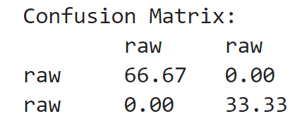
The model takes about 15 minutes to train, before spitting out results relating to the training in the form of a Confusion Matrix and a Precision, Recall, F1, and Accuracy Matrix. The Confusion Matrix highlights a highly effective model with 100% accuracy despite the imbalance of the data with 66% of the samples belonging to “Sports” and 33% belonging to “Business”.
We can also look at the Precision, Recall, F1, and Accuracy Matrix to see how the model performed at different neighbor counts (c), with both 1-NN and 3-NN performing the most accurately with the performance dropping off as more neighbors are considered.
With the model trained we can now evaluate its performance on unseen audio samples:
from pyAudioAnalysis import audioTrainTest as aT
aT.file_classification("file_loc/sports_podcast.wav", "data/knnSM","knn")

aT.file_classification("file_loc/business_podcast.wav", "data/knnSM","knn")

As we can see the model is performing well, in fact, if we evaluate it on the remaining 15 test podcast samples we get an accuracy of 100%. This indicates that the model is generally effective and that the feature extraction process created relevant data points that are useful for training models. This experiment on business and sports podcasts serves as more of a proof of concept however as the training set and test set we relatively small. despite the limitations, this example highlights the effectiveness of feature extraction from audio samples using PyAudio Analysis.
In Summary
Being able to extract relevant and useful data points from raw unstructured audio is an immensely useful process, especially for building effective classification models. PyAudio Analysis takes this feature extraction process and simplifies it into just a few lines of code you can execute on a directory of audio files to build your own classification models. If you are interested in learning more about PyAudio Analysis the Dolby.io team presented a tutorial on audio data extraction at PyData Global that included an introduction to the package, or you can read more about the package on its wiki here.
