
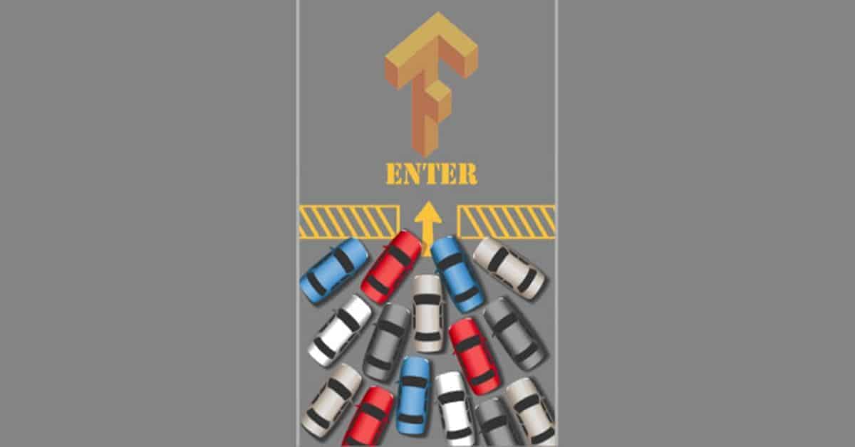
TensorFlow is one of Google’s flagship machine learning toolkits. Originally developed by researchers and engineers working on the Google Brain Team within Google’s Machine Intelligence research organization, Tensorflow found adoption in conducting machine learning and deep neural networks research. Subsequently, it was open sourced and is now available as a general purpose ML toolkit for a wide variety of applications. In this blog post, we will show you how to use the kNN routines of Tensorflow to solve a fundamental problem of city commuters, the traffic jams.
More...
Tensorflow is an open source software library for numerical computation using data flow graphs.It is Google’s attempt to put the power of Deep Learning into the hands of developers around the world.
The flexible architecture of Tensorflow allows you to deploy computation to one or more CPUs or GPUs in a desktop, server, or mobile device with a single API. It supports the popular Python programming language and is generic enough to be applicable in a wide variety of other domains.
Refer to the Getting Started Guide to take a dig at TensorFlow. If you are already familiar with it and are well aware of the k-NN routines supported, then head over to "Solving Practical Problem with kNN algorithm" to get the background on solving the real world problem that we are addressing in this post. To jump-start with the demo code & assets, take a look at "Building a Travel Time Recommendation Engine with TensorFlow."
What is kNN?
In pattern recognition, the k-nearest neighbor algorithm (k-NN) is a non-parametric method used for classification and regression. In both cases, the input consists of the k closest training examples in the feature space. Let's take a quick example to understand it better.
How does the KNN algorithm work ?
The below image shows the circles and rounded rectangles spread all over the graph. These represent two dominant classifications of data records in a dataset. For the sake of simplicity, let us assume that these are the only two classifications available in the dataset. Now, what if you have a test data record, the red diamond, and you want to find out which of these classes does this test sample belong to?

The “k” in k-NN algorithm is the count of nearest neighbors we wish to take a vote from. Let’s say k = 3. Hence, we make a circle with the diamond as the center and just big enough to enclose only three data points on the plane.

The three closest points to diamond are all circles, Hence with a good level of confidence, we can say that the diamond representing the test sample falls under circles class.
Solving a Practical Problem with kNN Algorithm
The above explanation of k-NN is a classification problem. We were trying to classify the test record (represented by the diamond point) into one of the two known classes, i.e., the circle or the rectangle.
However, kNN can also be used for regression problems. In such cases, we can predict one of the unknown parameters of the data record if other parameters are known. This way, kNN can predict outcomes to a particular event based on the event parameters being matched with historical outcomes of the same event.
One such event, which impacts our daily lives, is the act of commuting. As typical city dwellers, most of us commute every day for work, and often we run against the strict schedule. As an example, you need to head to the office tomorrow to attend an important early morning meeting. So you must start early and also ensure that the duration of commute, or the travel time, to your office is within that safe limit that ensures that you reach in time, neither late, nor too early.
What you need is a recommendation system that can suggest you the most favorable moment to leave from home so that you are assured of reaching the office, just in time. We have earlier presented a demo on how to build a recommendation engine that can optimize your travel time based on the dataset of historical travel times. We will take the same scenario here and descope the problem to focus only on the data, instead of building the entire application. And of course, we will show you how to use Tensorflow's kNN algorithm to solve this problem statement.
PROBLEM STATEMENT
How to predict the travel time between two locations within a city?
Datapoints Required for the Problem Statement
Within a city, the travel time from point A to B depends on many dynamic factors along with the demographics. Even within each hour of the day, there can be variations in travel time based on busy and non-busy hour traffic. Also, the day of the week plays a role, as the weekends will witness faster travel times due to low traffic density. Apart from this, there are also some environmental conditions, such as weather conditions and temperature that indirectly affect the travel time. So let’s consider these four data points that influence the travel time.
Datapoints affecting travel time
1. Time of the day
The travel time is largely dependent on this as during busy hours the traffic density on the city roads is at its peak.
2. Day of the week
Weekdays always witness more traffic density due to the rush of office commuters as compared to weekends.
3. Weather conditions
Harsh weather conditions can affect road and public infrastructure so this has an adverse impact on travel time.
4. Temperature
Extreme temperatures tend to keep people indoors which means less traffic density and faster travel.
Of course, the travel time is also dependent on the distance between the source and destination but for this discussion we are keeping that constant .
Sample Data for the Problem Statement
So we now have decided upon the four broad parameters that influence the travel time from a point A to point B. The next step is to collect some historical data that can aid in our prediction. This will be our training set to train our kNN algorithm. It will be used for predicting current travel time, based on the known parameters contained in a testing set, for the same route between point A to point B.
Dataset Jargon
Training set
Testing set
Training Set Composition
This training set will consist of the above four parameters along with the actual travel times, recorded from the past. We have collected the data for San Francisco between the two hospitals shown in the map.

Here is how the sample training set looks like. This is real data as has been captured using the Mapquest API.

This data is collected at 10:00 AM (Date column), on all Mondays(Day column) , for certain days between December 2015 & June 2016. The captured datapoints are
- Time of the day (Zone column) : A number code representing a 10 minute interval timezone, splitting the 24 hours of a day into 144 zones, ( For example, the 10 minute duration from 00:00 to 00:10 Hrs is coded as 1 and 00:10 to 00:20 Hrs is coded as 2, and so on)
- Day of the week (CodedDay column) : Week day in a coded number, 7 weekdays converted into to 7 numbers starting from 1(Sunday) to 7(Saturday).
- Weather Conditions (CodedWeather column) : Weather in a coded number. Check out the codes representing weather conditions that are used in this training set.
- Temperature (Temperature column) : Average temperature during the day, in Fahrenheit.
The training set also captures the actual time taken for travel in minutes (under the Realtime column) for each of the records that capture the four data points.
So in brief, here is the list of all six parameters that constitute one data record of the training set.
The starting time from the source or point A (represented by Date column)
Ten minute interval time zone of the day (represented by Zone column)
Day of the week (represented by Day and CodedDay column, both meaning the same)
Weather conditions on that day (represented by CodedWeather column)
The Temperature on that day (represented by Temperature column)
- The actual travel duration to reach destination, or point B, when someone started from the source at the time indicated in the Date column, (represented by Realtime column)
The Testing Set
The testing set looks like this.

It contains two records of the travel time dataset that has all the influencing factors that we explained earlier. The only thing left out is the travel time itself (the Realtime column from the training set). Why? Because this is the parameter that we will predict.
Building Subjective Insights on the Training Set
As humans, we are more inclined towards building subjective insights for arriving at decisions. The decision to start the commute at a particular time is also largely influenced by that. Based on our months or years of experience of commuting on the same route, we often choose to make our own judgment. But that judgment is always a rough guess.
Let’s assume for a moment that we have managed to gather this historical travel data contained in the training set. To make a decision out of that, we must decipher it first. If we plot this multidimensional data, then the resulting graph, plotted across a series of days, may look somewhat like this.

The immediate reaction that most people will have after viewing this graph would be a total sense of confusion.
Our brains cannot decipher so much data spanning across multiple dimensions. It is impossible to make a reasonably accurate prediction, even by plotting and visualizing this data. It's just way too complex.
Reducing Complexity for Arriving at Reasonable Predictions
Let’s simplify the plot to contain only the travel time and the weekday. Below is another plot of historical travel time. This one is a different route between Newark and Edison. Pay attention to the markings on the plot.

It is very clear that there is a definite shift in traffic patterns during weekdays and weekends. Looking at this graph, you can easily infer and make an approximate guess on the travel time based on the day of the week. But that guess is, at best, still a wish, that you hope to be true. That is the drawback of subjective insight.
Objective Insights for Accurate Prediction
A subjective decision based on a few historical experiences is a normal behavior for humans. Even if we have the graph and the data points at our disposal, we would still prefer to make an approximate decision based on some loosely concluded trends.
In reality, the data is too massive and multidimensional in nature. This complicates the decision making ability of humans. That's when we need to turn to computing machines with number crunching abilities to do the job for us.
Gaining Accuracy, One Dimension at a Time
Let's take a look at the training set again, but this time, with a different perspective. The following picture is a graph between the Coded Day and the Travel time. The blue color ‘x’ markers are the actual points that denote the travel times for a given day contained in the training set. Ignore the red color ‘o’ markers for now.

Now, imagine that you have to predict the travel time, based only on the knowledge of the day. Let's assume, you want to predict the travel time on Monday (CodedDay = 2) and Friday (CodedDay = 6), and so, you put the red dots on the plot to represent these two test points.
As you can witness from the plot, if you only have one known parameter, the day, then for a given day the travel time varies. You can see this from the vertical trail of 'x' marks for each day. In such cases, how would you know where to place the red dot? Considering this, the only prediction you can make is: "On Mondays, the travel time will range from 14 to 22 mins".

Expanding the plot to include one more known dimension ( either, time, weather or temperature) gets us a narrower range of predicted travel time, And the smaller the range gets, the more accurate is the prediction.
Likewise, we can expand this plot to include all the dimensions representing the four known data points and arrive at a practically accurate prediction. Unfortunately, the visualization of such multidimensional graph is very complex and becomes indecipherable for our brains. Hence let's just ignore it and head straight to the next section where we will use TensorFlow to do all the mathematical heavy lifting and generate predictions on the fly.
Building a Travel Time Recommendation Engine with Tensorflow
We will now show you how to leverage the objective insights that can be extracted from all the data points contained in training set to build a recommendation engine for predicting the travel time.
If you want to follow along, then ensure that you have the Python2 environment, preferably under Linux/Ubuntu, and make sure to install the TensorFlow library.
Now clone the GitHub repository to access the demo.

This repository contains the following demo assets
- TEST_SET.csv - Testing set
- TRAIN_SET.csv - Training set
- WeatherCodes.txt - Numeric codes for all weather conditions
- knn_tensor.py - Python demo program using the TensorFlow library to generate prediction.
Note on the Python Demo Program
If you are well versed with TensorFlow then you can have a look at the knn_tensor.py script to understand its nuances. Otherwise just follow along to witness WHAT the script does when it is executed. You can refer to the TensorFlow documentation later to learn the HOWs of it.
Executing the Demo Program
Run the knn_tensor.py script to get the prediction. ( make sure you have permissions for executing the script).
“python knn_tensor.py”

The script reads through the training set to build the prediction model and spews out some numbers. Let's find out how do we arrive at these numbers for predicted travel time.
Verification of Predicted Travel Time
Let's verify the prediction results using the first principle method. Since the training set is small in our case, this can be easily achieved by matching the predicted result with the records in training set.
The testing set has two records. The first test record (Test 0 as per the program output) contains the following parameter values.
- CodedDay : 2
- CodedWeather : 30
- Temperature : 48
- Zone : 61
Note :- Let’s ignore the second record for the moment. The python program is written in a way that it can output multiple predictions based on the multiple test records in testing set. For now, we will ignore all but the first record only (Test 0)
So with the above test record in the TEST_SET.csv , the program output is.
As you can see, the predicted travel time for Test 0 is 19.98 mins. To verify this, let's compare the test data with training data.

In the image above, we have lined up the records in training set with that of testing set. You can see that the test data for first record of the testing set has the exact same parameter values in the training set as well (see the highlighted rows). Hence this becomes a straight forward prediction, where we get the exact prediction based on the exact same historical conditions.
Now lets, modify the TEST_SET.csv to change the first row of test record as follows
- CodedDay : 2
- CodedWeather : 23
- Temperature : 48
- Zone : 61
We have changed CodedWeather to 23. Rest all values remain same. With this, we get the following output.
OK, so now let's see how we arrived at a prediction of 20.18 mins for Test 0.
If you browse through the TRAIN_SET.csv, you will not find any record whose parameters all match with the test 0's test data in TEST_SET.csv . The closest match is as shown below in the highlighted rows.

As you can see, the Zone, CodedDay and CodedWeather values in the test record matches with training set, but the temperature does not match. Therefore, we do not have an exact match of all the four influencing parameters of the test record with any of the records in the entire training set.
In this case, the TensorFlow’s kNN algorithm calculates the nearest approximate and declares the temperature value of 52, in the training set as the closest neighbor to 48, with all other parameters remaining same. Hence the prediction, 20.18.
Make Your Own Predictions Now
You can change the parameters in testing set as per your wish and give it a try now. Try to verify the results by matching the two datasets and see if it makes sense. In the process, you may experience some interesting observations which we have not addressed in this post.
We have not covered anything about the kNN algorithm's configuration w.r.t TensorFlow and its behavior. If you are curious, you can look up the documentation to tweak the python program and get different results. A complete explanation of this demands a separate post which we will plan sometime in the future. But for now, play around with the script and data and make your own predictions.
If you want to make a practical use of this demo, then you can also use your phone to manually record your travel time and all the four influencing factors, for each day, for a period of one month, along the route from your home to office. Build your training set from that data and then you are good to go. If you are really interested to know how to build a real recommendation engine out of this, then check out this blog post.

wow that is one excellent post
Thanks for the appreciation. Glad you liked it.
Thanks, nice introduction for traffic prediction with ML
Thanks
Nice illustration. I am also working on this domain sir. Shall I contact you through mail Sir