How to Turn Timescale Cloud into an Observability Backend With Promscale

The adoption of modern cloud-native distributed architectures has grown dramatically over the last few years, due to the great advantages they present if compared with traditional, monolithic architectures – like flexibility, resilience against failure, or scalability. However, the price we pay is an increased degree of complexity. Operating cloud-native microservices environments is hard: in particular, the dynamic nature of those systems makes it difficult to predict failure patterns, leading to the emergence of observability as a practice.

This article was originally published in Timescale.

The promise of observability is to help engineering teams quickly identify and fix those unpredicted failures when they occur in production, ideally before they impact users. This gives engineering teams the ability to deliver new features frequently and with confidence.

A requirement to get the benefits of observability is to have access to comprehensive telemetry about our systems, and this requires those systems to be instrumented. Luckily, we have great open-source options available that make instrumentation easier – particularly, Prometheus exporters and OpenTelemetry instrumentation.

Once a system is instrumented, we need a way to efficiently store and analyze the telemetry it generates. And since modern systems typically have a lot more components than traditional ones, and since we have to collect telemetry about each of these systems to ensure we can effectively identify problems in production, we end up having to manage large amounts of data….

For this reason, the data layer is usually the most complex component of an observability stack – especially at scale. Often, storing observability data gets too complex or too expensive; plus, it can also get complicated to extract value from it, as it may be non-trivial how to analyze this data. If that’s your experience, you won’t be getting the full benefits of observability.

In this blog post, we explain how you can use Timescale Cloud and Promscale to store and analyze telemetry data from your systems instrumented with Prometheus and OpenTelemetry.

Timescale Cloud is a database cloud built on PostgreSQL and TimescaleDB; built to store massive volumes of time series data, Timescale Cloud is an ideal option to store your observability data efficiently – with features like native columnar compression, flexible pricing plans with decoupled compute and storage, and downsampling capabilities through continuous aggregates.

Promscale is an open-source observability backend built on PostgreSQL and TimescaleDB that automatically infers a schema to store metrics and traces, allowing you to analyze them as you would do with any other relational table in PostgreSQL: using SQL. Promscale has native support for Prometheus metrics and OpenTelemetry traces, as well as many other formats like StatsD, Jaeger, and Zipkin through the OpenTelemetry Collector (and it is also 100% PromQL compliant!). Promscale also easily integrates with tools like Grafana and Jaeger.

Used together, Promscale and Timescale Cloud are powerful allies:

• Get started in minutes. To create a service in Timescale Cloud takes one click, and by using tobs (our CLI tool), you can install not only Promscale – but your complete observability stack (Promscale, Jaeger, Grafana, and Prometheus) with a single command.
• Worry-free operations. Managing the data layer at scale in production is complex. It requires you to perform maintenance tasks and backups, scale the system by adding new nodes as your needs grow or set up tools and procedures to bring the system back up when it goes down. With Timescale Cloud all of that is taken care of for you.
• Native integration with Prometheus and OpenTelemetry. Promscale seamlessly integrates with Prometheus and OpenTelemetry to transform Timescale Cloud into a long-term storage for metrics and traces with support for Prometheus multi-tenancy and OpenMetrics exemplars. Even more, Promscale also provides full PromQL support!
• Get unprecedented insights from your metrics and traces. Use the power of standard SQL (and of TimescaleDB’s advanced analytic functions) to query and correlate metrics, traces, and business data together. You can ask complex questions to troubleshoot your systems effectively, building powerful Grafana dashboards using plain SQL queries.
• The scalability of TimescaleDB and the rock-solid foundation (and compatibility!) of PostgreSQL. Timescale Cloud supports up to 16 TB storage plans, with horizontal scalability, one-click creation of multi-node databases, one-click database resizing without downtime, one-click database forking, storage autoscaling, and much more – with all the advantages (and the peace of mind) of a technology built on PostgreSQL. You can enjoy the large ecosystem of PostgreSQL integrations, including data visualization tools, AI platforms, IDEs, and ORMs.

This blogpost will walk you through everything you need to know about integrating Timescale Cloud and Promscale in a Kubernetes-based system. It will also give you further insights on how to optimally configure Prometheus, OpenTelemetry, Grafana, and Jaeger – giving you examples of how you can use SQL to analyze your metrics and traces. 🔥

If you are new to Timescale, join the TimescaleDB Community on Slack and chat with us about observability, Promscale, Timescale Cloud, or anything in between. Plus, we just launched our Timescale Community Forum! If you have a technical question in mind that may need a bit of a deeper answer, the forum will be the perfect medium for you.

Integrating the Promscale Connector with Timescale Cloud

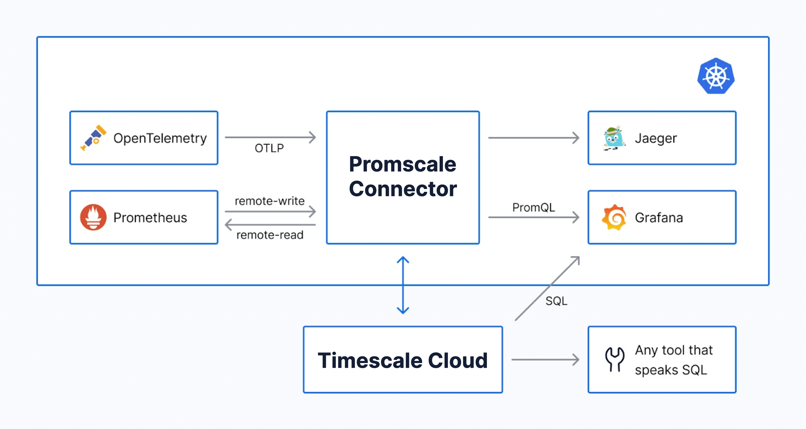
The architecture of the observability backend based on Promscale and Timescale Cloud is quite simple, having only two components:

• The Promscale Connector. This is the stateless service that provides the ingest interfaces for observability data, processing that data appropriately to store it in a SQL-based database. It also provides an interface to query the data with PromQL. The Promscale Connector ingests Prometheus metrics, metadata, and OpenMetrics exemplars using the Prometheus remote_write interface. It also ingests OpenTelemetry traces using the OpenTelemetry protocol (OTLP). It can also ingest traces and metrics in other formats using the OpenTelemetry Collector. For example, you can use the OpenTelemetry Collector with Jaeger as the receiver and OTLP as the exporter to ingest Jaeger traces into Promscale.
• A Timescale Cloud service (i.e. a cloud TimescaleDB database). This is where we will store our observability data, which will already have the appropriate schema thanks to the processing done by the Promscale Connector.

Creating a Timescale Cloud Service

Before diving into the Promscale Connector, let’s first create a Timescale Cloud service  (i.e., a TimescaleDB instance) to store our observability data:

1. If you are new to Timescale Cloud, create an account (free for 30 days, no credit card required) and log in.
2. Once you’re in the Services page, click on “Create service” in the top right, and select “Advanced options”.
3. A configuration screen will appear, in which you will be able to select the compute and storage of your new service. To store your observability data, we recommend that you allocate a minimum of 4 CPUs, 16GB of Memory, and 50GB of disk (equivalent to 840GB of uncompressed data) as a starting point. You can scale up this setup as you need it, once your data ingestion and query rate increase.
4. Once you’re done, click on “Create service”.
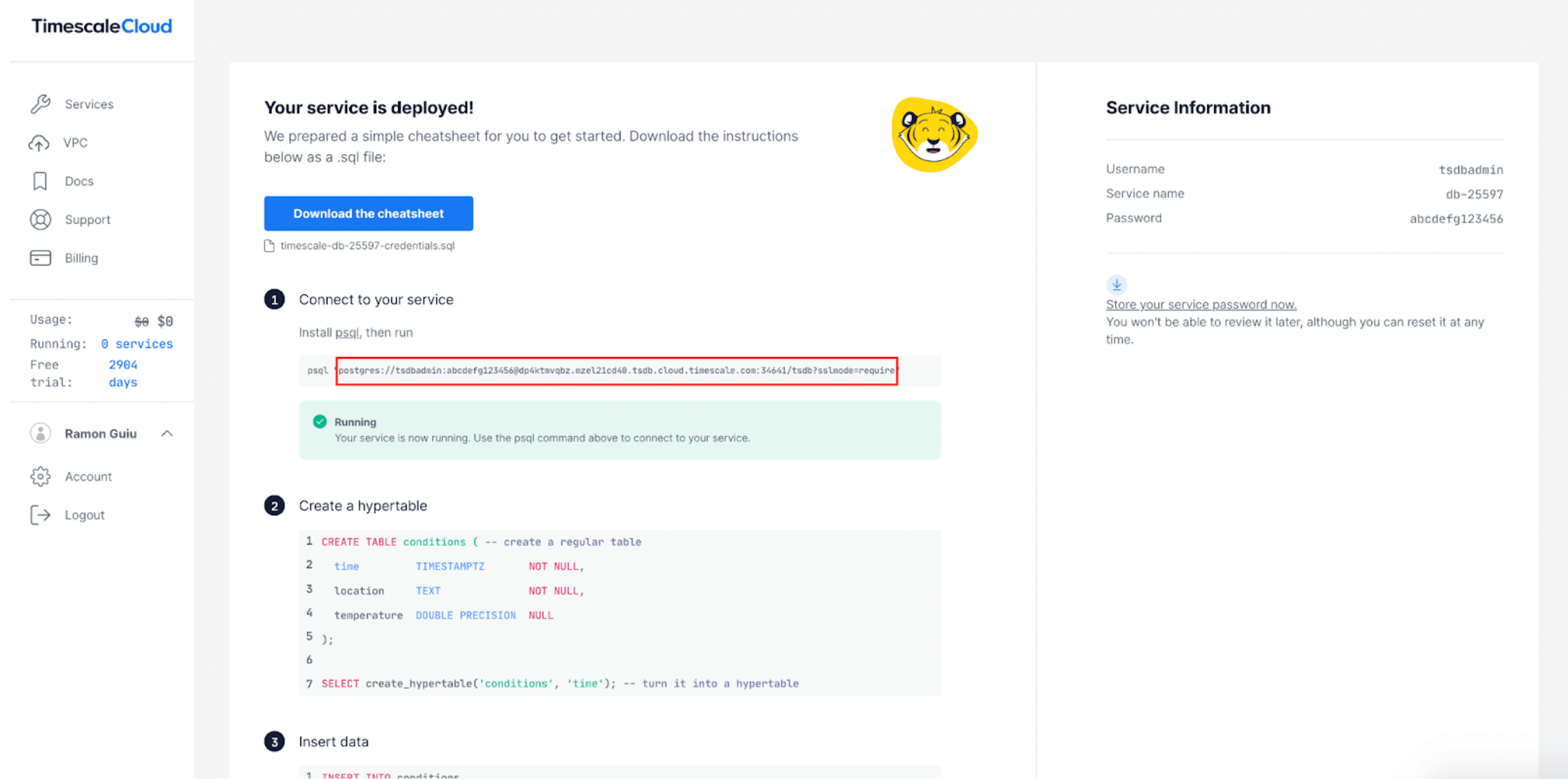
5. Wait for the service creation to complete, and copy the service URL highlighted with the red rectangle in the screenshot below. You will need it later!

Now that your Timescale Cloud service is ready, it is time to deploy the Promscale Connector on your Kubernetes cluster. We will discuss two different deployment options:

• Installing Promscale using tobs (The Observability Stack for Kubernetes). If you are not yet using Prometheus and OpenTelemetry in your Kubernetes cluster, this is our recommended method, as tobs will also install and automatically configure Grafana, Jaeger, and Prometheus in your Kubernetes cluster with a single command.
• Installing Promscale manually through a Kubernetes manifest. You can use this option if you are already running Prometheus or OpenTelemetry in your Kubernetes cluster. Compared to the tobs approach, this will require that you manually configure the existing Prometheus, OpenTelemetry, Grafana and Jaeger to connect to Promscale.

Installing Promscale Using TOBS (The Observability Stack for Kubernetes)

Tobs is a CLI that makes it simple to install a full observability stack into a Kubernetes cluster, including:

• Kube-Prometheus
• Promscale
• TimescaleDB (In this blog post, since we are using a Timescale cloud service, a local TimescaleDB instance will not be deployed by tobs)
• Promlens
• Opentelemetry-Operator
• Jaeger

Tobs makes it much easier to deploy and manage an observability stack: with tobs, you are just one command away from getting the complete stack up and running. Tobs includes both a CLI tool and a helm-chart combining the open-source projects that are listed above, and it takes care of directly connecting all these components out-of-the-box, giving them the appropriate configuration tobs also configures the Prometheus, Jaeger, and PostgreSQL data sources in Grafana for you.

To install the observability stack using tobs, follow these steps:

  curl --proto '=https' --tlsv1.2 -sSLf  https://tsdb.co/install-tobs-sh |sh

• Make sure you move the tobs binary from its current directory to your /bin directory, or add it to your PATH.
• Deploy the observability stack using tobs install. Through the command below, we are also adding three more steps:
  • We will connect the Promscale Connector to Timescale Cloud through the service URL you obtained when you created it.
  • We will enable tracing support by adding the feature flag –tracing. (Support for tracing is in beta at the moment, and therefore it needs to be explicitly enabled).

tobs install --tracing --external-timescaledb-uri <service-url>

• You will be asked for permission to install the cert-manager (unless it already exists in the cluster). If so, type yes.
• Once the installation is complete, you are done – you have a full observability stack ready! Jump straight to the sections on Prometheus, Grafana, and Jaeger to see how you can access and configure these tools.

Accessing Grafana

One of the advantages of using SQL-compatible backend for observability is that you can build dashboards using plain SQL through tools like Grafana, allowing you to get deeper insights into your data than if using only Jaeger. We’re planning to publish more content on how to use SQL to build awesome visualizations for metrics and traces (stay tuned ✨), but if you are interested in getting some tips right away, check out our blog and YouTube series on Grafana.

If you have deployed Promscale using tobs, you already have Grafana fully installed and configured in your Kubernetes cluster, and no further action is required from you. To access Grafana, simply follow these steps:

• Get the Grafana password:

tobs grafana get-password

• Port forward Grafana to localhost:8080

# Port forward Grafana to localhost:8080
tobs grafana port-forward

# Open localhost:8080 in your browser

• Open localhost:8080 in your browser
• Log in using “admin” as username and the password you just retrieved

You will see that tobs has automatically added three data sources to Grafana:

• A Prometheus data source, so you can query Prometheus metrics using PromQL.
• A Jaeger data source, so you can visualize your traces in Grafana’s distributed tracing UI.
• A PostgreSQL data source, so you can use SQL to query the metrics and traces stored in Promscale (as well as all your other tables and hypertables hosted in your Timescale Cloud service).

Accessing Jaeger

You can also visualize the traces stored in Promscale in Jaeger, an open-source tool for visualizing distributed traces. In order for the Jaeger Query to show traces stored in Promscale, we leverage Jaeger’s gRPC based backend store integration.

Using tobs, you already have Jaeger installed. To access it, do the following:

# Port forward Jaeger to localhost:16686
tobs jaeger port-forward

# Open localhost:16686 in your browser

Installing Promscale Using a Kubernetes Manifest

If you are already running Prometheus and/or OpenTelemetry in your Kubernetes cluster, you may prefer to use the Kubernetes manifest below – which will only install the Promscacle Connector. (The Promscale Connector is a single stateless service, so all you have to deploy is the Connector and the corresponding Kubernetes service.)

Note: Remember to replace <DB-URI> with the service URL from your Timescale Cloud service.

---
# Source: promscale/templates/service-account.yaml
apiVersion: v1
kind: ServiceAccount
automountServiceAccountToken: false
metadata:
  name: promscale
  namespace: default
  labels:
    app: promscale
    app.kubernetes.io/name: "promscale-connector"
    app.kubernetes.io/version: 0.8.0
    app.kubernetes.io/part-of: "promscale-connector"
    app.kubernetes.io/component: "connector"
---
# Source: promscale/templates/secret-connection.yaml
apiVersion: v1
kind: Secret
metadata:
  name: promscale
  namespace: default
  labels:
    app: promscale
    app.kubernetes.io/name: "promscale-connector"
    app.kubernetes.io/version: 0.8.0
    app.kubernetes.io/part-of: "promscale-connector"
    app.kubernetes.io/component: "connector"
stringData:
  PROMSCALE_DB_URI: "<DB-URI>"
---
# Source: promscale/templates/svc-promscale.yaml
apiVersion: v1
kind: Service
metadata:
  name: promscale-connector
  namespace: default
  labels:
    app: promscale
    app.kubernetes.io/name: "promscale-connector"
    app.kubernetes.io/version: 0.8.0
    app.kubernetes.io/part-of: "promscale-connector"
    app.kubernetes.io/component: "connector"
spec:
  selector:
    app: promscale
  type: ClusterIP
  ports:
  - name: metrics-port
    port: 9201
    protocol: TCP
  - name: traces-port
    port: 9202
    protocol: TCP   
---
# Source: promscale/templates/deployment-promscale.yaml
apiVersion: apps/v1
kind: Deployment
metadata:
  name: promscale
  namespace: default
  labels:
    app: promscale
    app.kubernetes.io/name: "promscale-connector"
    app.kubernetes.io/version: 0.8.0
    app.kubernetes.io/part-of: "promscale-connector"
    app.kubernetes.io/component: "connector"
spec:
  replicas: 1
  strategy:
    type: Recreate
  selector:
    matchLabels:
      app: promscale
  template:
    metadata:
      labels:
        app: promscale
        app.kubernetes.io/name: "promscale-connector"
        app.kubernetes.io/version: 0.8.0
        app.kubernetes.io/part-of: "promscale-connector"
        app.kubernetes.io/component: "connector"
      annotations: 
        prometheus.io/path: /metrics
        prometheus.io/port: "9201"
        prometheus.io/scrape: "true"
    spec:
      containers:
        - image: timescale/promscale:0.8.0
          imagePullPolicy: IfNotPresent
          name: promscale-connector
          args:
            - -otlp-grpc-server-listen-address=:9202
            - -enable-feature=tracing
          envFrom:
          - secretRef:
              name: promscale
          ports:
            - containerPort: 9201
              name: metrics-port
            - containerPort: 9202
              name: traces-port
      serviceAccountName: promscale

To deploy the Kubernetes manifest above, run:

kubectl apply -f <above-file.yaml>

And check if the Promscale Connector is up and running:

kubectl get pods,services --selector=app=promscale

Configuring Prometheus

Prometheus is a popular open-source monitoring and alerting system that can be used to easily and cost-effectively monitor modern infrastructure and applications. However, Prometheus is not focused on advanced analytics –  by itself, Prometheus doesn’t provide durable, highly-available long-term storage.

One of the top advantages of Promscale is that it integrates seamlessly with Prometheus for the long-term storage of metrics. Apart from its 100% PromQL compliance, multitenancy, and OpenMetrics exemplars support, Promscale allows you to use SQL to analyze your Prometheus metrics: this enables more sophisticated analysis than what you’d usually do in PromQL, making it easy to correlate your metrics with other relational tables for an in-depth understanding of your systems.

Manually configuring Promscale as remote storage for Prometheus only requires a quick change in the Prometheus configuration. To do so, open the Prometheus configuration file, and add or edit these lines:

remote_write:
  - url: "http://promscale-connector.default.svc.cluster.local:9201/write"
remote_read:
  - url: "http://promscale-connector.default.svc.cluster.local:9201/read"
    read_recent: true

Check out our documentation for more information on how to configure the Prometheus remote-write settings to maximize Promscale metric ingest performance!

Configuring OpenTelemetry

Our vision for Promscale is to enable developers to store all observability data (metrics, logs, traces, metadata, and other future data types) in a single mature, open-source, and scalable store based on PostgreSQL, so they can use a unified interface to analyze all their data.

Getting one step closer to that vision, Promscale includes the beta support for OpenTelemetry traces. Promscale exposes an ingest endpoint that is OTLP-compliant, enabling you to directly ingest OpenTelemetry data, while other tracing formats (like Jaeger, Zipkin, or OpenCensus) can also be sent to Promscale through the OpenTelemetry Collector.

If you want to learn more about traces in Promscale,  Ramon Guiu (VP of Observability in Timescale) and Ryan Booz (Director of Developer Advocacy) chat about traces, OpenTelemetry, and our vision for Promscale in the stream below:

To manually configure the OpenTelemetry collector, we will add Promscale as the OTLP backend store for ingesting the traces that are emitted from the collector, establishing Promscale as the OTLP exporter endpoint:

exporters:
  otlp:
    endpoint: "promscale-connector.default.svc.cluster.local:9202"
    insecure: true

Note: In the above OTLP exporter configuration, we are disabling TLS setting insecure to true for the demo purpose. You can enable TLS by configuring certificates at both OpenTelemetry-collector and Promscale. In TLS authentication Promscale acts as the server.

To export data to an observability backend in production, we recommend that you always use the OpenTelemetry Collector. However, for non-production setups, you can also send data from the OpenTelemetry instrumentation libraries and SDKs directly to Promscale using OTLP. In this case, the specifics of the configuration depend on each SDK and library – see the corresponding GitHub repository or the OpenTelemetry documentation for more information.

Installing Jaeger Query

Since our recent contribution to Jaeger, it now supports querying traces from a compliant remote gRPC backend store in addition to the local plugin mechanism – so you can now directly use upstream Jaeger 1.30 and above to visualize traces from Promscale, without the need to deploy our Jaeger storage plugin. A huge thank you to the Jaeger team for accepting our PR!

In Jaeger, you can use the filters in the left menu to retrieve individual traces, visualizing the sequence of spans that make up an individual trace. This is useful to troubleshoot individual requests.

To deploy the Jaeger query and Jaeger query service, use the manifest below:

---
# Jaeger Promscale deployment
apiVersion: apps/v1
kind: Deployment
metadata:
  name: jaeger
  namespace: default
  labels:
    app: jaeger
spec:
  replicas: 1
  selector:
    matchLabels:
      app: jaeger
  template:
    metadata:
      labels:
        app: jaeger
    spec:
      containers:
        - image: jaegertracing/jaeger-query:1.30
          imagePullPolicy: IfNotPresent
          name: jaeger
          args:
          - --grpc-storage.server=promscale-connector.default.svc.cluster.local:9202
          - --grpc-storage.tls.enabled=false
          - --grpc-storage.connection-timeout=1h
          ports:
            - containerPort: 16686
              name: jaeger-query
          env:
            - name: SPAN_STORAGE_TYPE
              value: grpc-plugin
---
# Jaeger Promscale service
apiVersion: v1
kind: Service
metadata:
  name: jaeger
  namespace: default
  labels:
    app: jaeger
spec:
  selector:
    app: jaeger
  type: ClusterIP
  ports:
  - name: jaeger
    port: 16686
    targetPort: 16686
    protocol: TCP

To deploy the manifest, run:

kubectl apply -f <above-manifest.yaml>

Now, you can access Jaeger:

# Port-forward Jaeger service
kubectl port-forward svc/jaeger 16686:16686

# Open localhost:16686 in your browser

Configuring Data Sources in Grafana

As shown in the screenshot below, in order to manually configure Grafana, we’ll be adding three data sources: Prometheus, Jaeger, and PostgreSQL. (As a reminder, if you used tobs to install the stack, these data sources are automatically added and configured for you.)

Configuring the Prometheus Data Source in Grafana

• In Grafana navigate to Configuration → Data Sources → Add data source → Prometheus.
• Configure the data source settings:
  • In the Name field, type Promscale-Metrics.
  • In the URL field, type http://promscale-connector.default.svc.cluster.local:9201, using the Kubernetes service name of the Promscale Connector instance. The 9201 port exposes the Prometheus metrics endpoints.
  • Use the default values for all other settings.

Note: If you are running Grafana outside the Kubernetes cluster where Promscale is running, do not forget to change the Promscale URL to an externally accessible endpoint from Grafana.

Once you have configured Promscale as a Prometheus data source in Grafana, you can create panels that are populated with data using PromQL as in the screenshot below:

Configuring the Jaeger Data Source in Grafana

In Grafana navigate to Configuration → Data Sources → Add data source → Jaeger.

• Configure the data source settings:
  • In the Name field, type Promscale-Traces.
  • In the URL field, type http://jaeger.default.svc.cluster.local:16686, using the Kubernetes service endpoint of the Jaeger Query instance.
  • Use the default values for all other settings.

Note: The Jaeger data source in Grafana uses the Jaeger Query endpoint as the source, which in return queries the Promscale Connector to visualize the traces: Jaeger data source in Grafana -> Jaeger Query -> Promscale.

You can now filter and view traces stored in Promscale using Grafana. To visualize your traces, go to the “Explore” section of Grafana. You will be taken to the traces filtering panel.

Configuring the PostgreSQL Data Source in Grafana

In Grafana navigate to Configuration → Data Sources → Add data source → PostgreSQL.

• Configure the data source settings:
  • In the Name field, type Promscale-SQL.
  • In the Host field, type <host>:<port>, where host and port need to be obtained from the service url you copied when you created the Timescale cloud service. The format of that url is postgresql://[user[:password]@][host][:port][/dbname][?param1=value1&…]
  • In the Database field, type the dbname from the service url.
  • In the User and Password fields, type the user and password from the service.
  • Change the TLS/SSL Mode to require as the service url by default contains the TLS mode as required.
  • Change the TLS/SSL Method File system path.
  • Use the default values for all other settings.
  • In the PostgreSQL details section enable the TimescaleDB option.

kg-card-end: markdown

You can now create panels that use Promscale as a PostgreSQL data source, using SQL queries to feed the charts:

Using SQL to Query Metrics and Traces

A powerful advantage of transforming Prometheus metrics and OpenTelemetry traces into a relational model is that developers can use the power of SQL to analyze their metrics and traces.

In the case of traces, this is especially relevant. Even if traces are essential to understanding the behavior of modern architectures, tracing has seen significantly less adoption than metrics monitoring – at least, until now. One of the reasons behind this low adoption were the difficulties associated with instrumentation, a situation that has improved considerably thanks to OpenTelemetry. However, traces were also problematic in another way: even after doing all the instrumentation work, developers realized that there is no clear way to analyze tracing data through open-source tools. For example, tools like Jaeger offer a fantastic UI for the basic filtering and visualizing of individual traces, but they don’t allow analyzing data by running arbitrary queries or in aggregate to identify behavior patterns.

In other words, many developers felt that adopting tracing was not worth the effort, considering the value of the information they could get from them. Promscale aims to solve this problem by giving developers a familiar interface for exploring their observability data, which now have the ability to use joins, sub-queries, and all the advantages of the SQL language.

In this section, we’ll be showing you a few examples of queries you could use to get direct value not only from your OpenTelemetry traces but also from your Prometheus metrics. Promscale is 100% PromQL-compliant, but the ability to query Prometheus with SQL helps you answer questions that are not possible to answer with PromQL.

Querying Prometheus Metrics With SQL

Example 1: Visualize the metric go_gc_duration_seconds in Grafana

In order to visualize such metric in Grafana, we would build a panel using the following query:

SELECT
  jsonb(v.labels)::text as "metric",
  time AS "time",
  value as "value"
FROM "go_gc_duration_seconds" v
WHERE
  $__timeFilter("time")
ORDER BY 2, 1

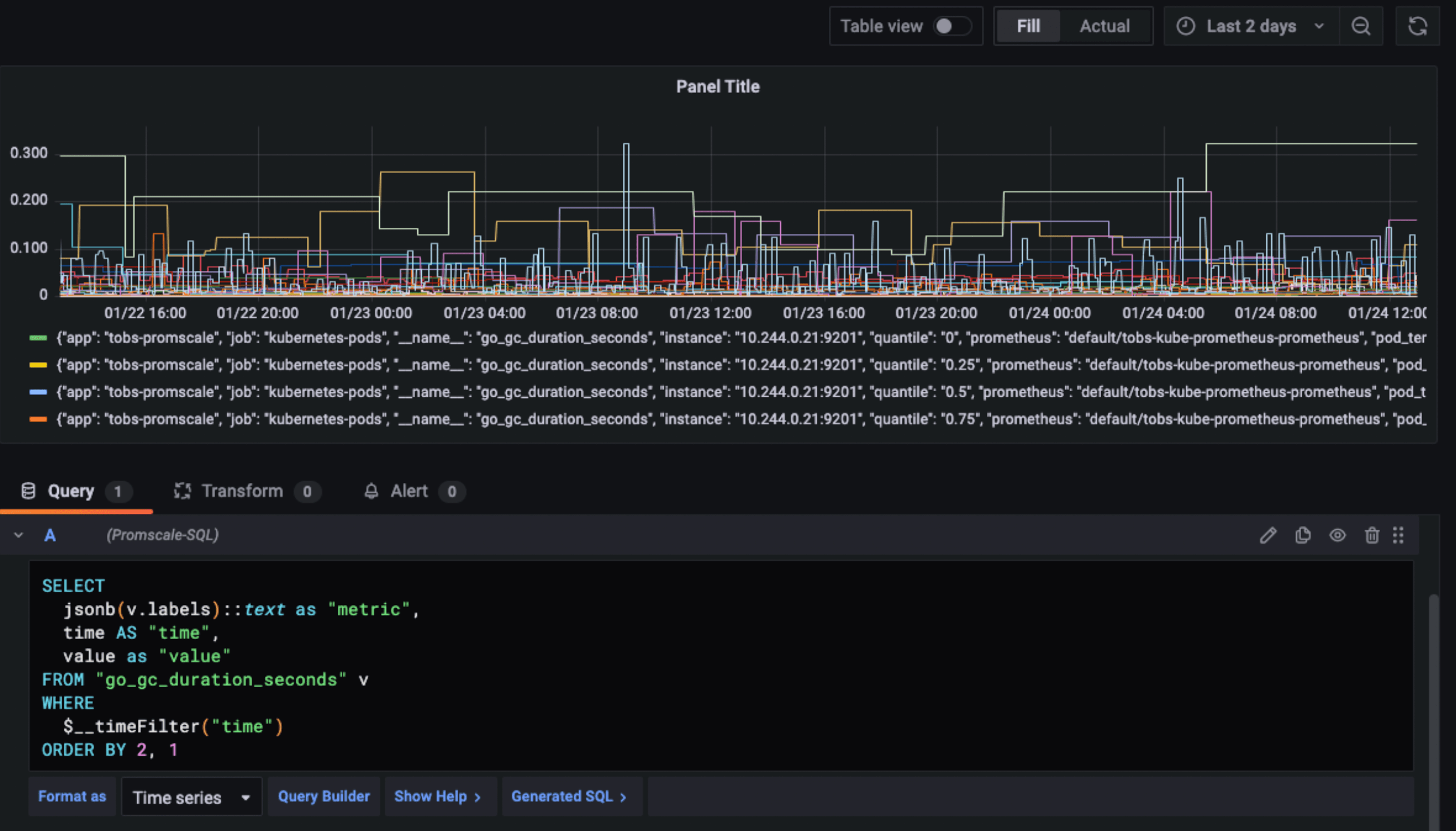
The result would look like this:

Example 2: Calculate the 99th percentile over both time and series (pod_id) for the metric go_gc_duration_seconds

This metric is a measurement for how long garbage collection is taking in Go applications. This is the query:

SELECT 
   val(pod_id) as pod, 
   percentile_cont(0.99) within group(order by value) p99 
FROM 
   go_gc_duration_seconds 
WHERE 
   value != 'NaN' AND val(quantile_id) = '1' AND pod_id > 0 
GROUP BY 
   pod_id 
ORDER BY 
   p99 desc;

And this is the result:

Want more examples on how to query metrics with SQL? Check out our docs. ✨

Querying OpenTelemetry Traces With SQL

Example 1: Show the dependencies of each service, the number of times the dependency services have been called, and the time taken for each request

As we said before, querying traces can tell you a lot about your microservices. For example, look at the following query:

SELECT
    client_span.service_name AS client_service,
    server_span.service_name AS server_service,
    server_span.span_name AS server_operation,
    count(*) AS number_of_requests,
    ROUND(sum(server_span.duration_ms)::numeric) AS total_exec_time
FROM
    span AS server_span
    JOIN span AS client_span
    ON server_span.parent_span_id = client_span.span_id
WHERE
    client_span.start_time > NOW() - INTERVAL '30 minutes' AND
    server_span.start_time > NOW() - INTERVAL '30 minutes' AND
    client_span.service_name != server_span.service_name
GROUP BY
    client_span.service_name,
    server_span.service_name,
    server_span.span_name
ORDER BY
    server_service,
    server_operation,
    number_of_requests DESC;

Now, you have the dependencies of each service, the number of requests, and the total execution time organized in a table:

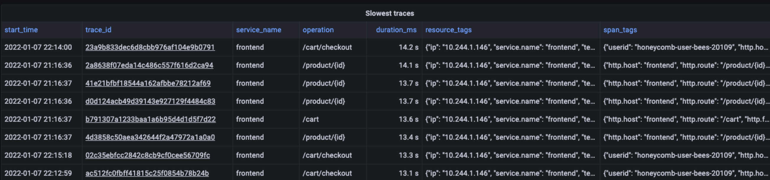
Example 2: List the top 100 slowest traces

A simple query like this would allow you to quickly identify requests that are taking longer than normal, making it easier to fix potential problems.

SELECT
  start_time,
  replace(trace_id::text, '-', '') as trace_id,
  service_name,
  span_name as operation,
  duration_ms,
  jsonb(resource_tags) as resource_tags,
  jsonb(span_tags) as span_tags
FROM span
WHERE
  $__timeFilter(start_time) AND
  parent_span_id = 0
ORDER BY duration_ms DESC
LIMIT 100

You can also do this with Jaeger – however, the sorting is done after retrieving the list of traces, which is limited to a maximum of 1,500. Therefore, if you have more traces, you could be missing some of the slowest ones in the results.

The result would look like the table below:

Example 3: Plot the p99 response time for all the services from traces

The following query uses TimescaleDB’s approx_percentile to calculate the 99th percentile of trace duration for each service by looking only at root spans (parent_span_id = 0) reported by each service. This is essentially the p99 response time by service as experienced by clients outside the system:

SELECT
    time_bucket('1 minute', start_time) as time,
    service_name,
    ROUND(approx_percentile(0.99, percentile_agg(duration_ms))::numeric, 3) as p99
FROM span
WHERE
     $__timeFilter(start_time) AND
     parent_span_id = 0
GROUP BY time, service_name;

To plot the result in Grafana, you would build a Grafana panel with the above query, configuring the data source as Promscale-SQL and selecting the format as “time series”.

It would look like this:

Getting Started

If you are new to Timescale Cloud and Promscale,

• Create a Timescale Cloud account (free for 30 days, no credit card required).
• Deploy a full open-source observability stack into your Kubernetes cluster by using tobs, our CLI. Apart from Promscale, you will also get to tools like Prometheus, Grafana, OpenTelemetry, and Jaeger – fully configured and ready to go 🔥
• Check out our documentation for more information on the architecture of Promscale, Prometheus, and OpenTelemetry. You will also find tips for querying and visualizing data in Promscale.
• Check out the Promscale GitHub repo. Promscale is open-source and completely free to use. (GitHub ⭐️ ‘s and contributions are welcome and appreciated! 🙏)
• Explore our YouTube Channel for tutorials on Timescale Cloud, TimescaleDB features like compression and continuous aggregates, Promscale, and much more!

And whether you’re new to Timescale or an existing community member, we’d love to hear from you! Join us in our Community Slack: this is a great place to ask any questions on Timescale Cloud or Promscale, get advice, share feedback, or simply connect with the Timescale engineers. We are 8K+ and counting!