

This post explains how to perform text recognition from images.
This post was originally published in Weights & Biases.
Text Extraction: Introduction
Extracting text of various sizes, shapes, and orientations from images is an essential problem in many contexts, especially in e-commerce, augmented reality assistance systems, and content moderation in social media platforms. To tackle this problem, one needs to accurately extract the text from images. Basically, text extraction can be achieved into two steps, i.e., text detection and text recognition or by training a single model to achieve both text detection and recognition like: A single Neural Network for Text Detection and Text Recognition. In this post, I will mainly be explaining the former approach.
Get the full code here.
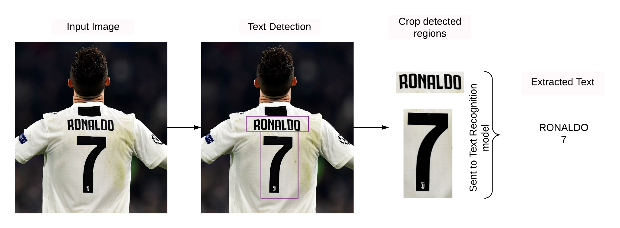
- Text detection helps identify the region in the image where the text is present. It takes in an image as an input, and the outputs bounding boxes.
- Text recognition extracts the text from the input image using the bounding boxes obtained from the text detection model. It takes in an image and some bounding boxes as inputs and outputs some raw text.
Text detection is very similar to the object detection task where the object which needs to be detected is nothing but the text. Much research has taken place in this field to detect text out of images accurately, and many of these detectors detect text at the word level. Few of the examples are:
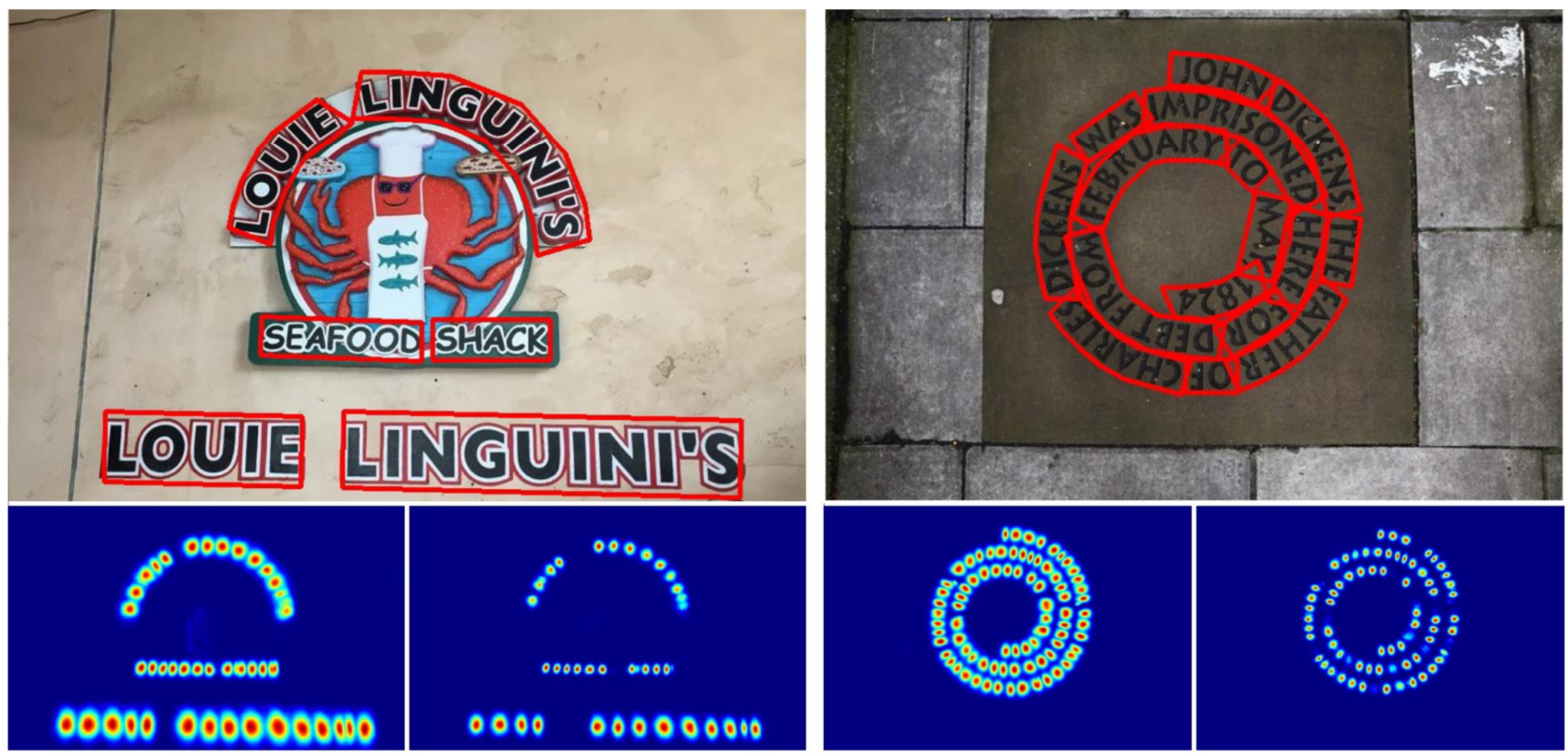
However, the problem with word-level detectors is that they fail to detect words of arbitrary shape.
Recent work published in CVPR 2019, Character Region Awareness for Text Detection by Youngmin et al., has shown that detecting text area by exploring each character and affinity between characters helps to detect arbitrarily shaped texts. Few examples can be seen below:
In this report, I will mainly focus on explaining the CRNN-CTC network for text recognition. For text detection, you can use any of the techniques mentioned above based on the complexity of the use case that you have in hand.
Text Recognition Pipeline
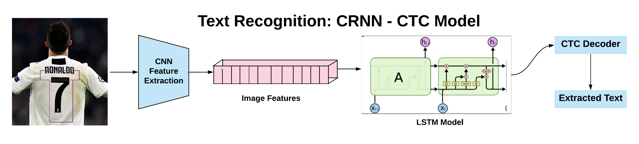
After the text detection step, regions, where the text is present, are cropped and sent through convolutional layers to get the features from the image. Later these features are fed to many-to-many LSTM architecture, which outputs softmax probabilities over the vocabulary. These outputs from different time steps are fed to the CTC decoder to finally get the raw text from images. I will discuss in detail each of the steps in the further sections of the report. Let’s first understand the concept of receptive fields, making it easier to understand how features from the CNN model are fed to the LSTM network.
Receptive Fields
The receptive field is defined as the region in the input image/space that a particular CNN’s feature is looking at.
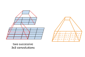
Let us say we have an input image of the shape 5 x 5 and a filter 3 x 3. As seen from the above image, after applying a filter on the input image, the feature map’s value has visibility on the 3 x 3 patch of the image. If we move to the second layer, 3 x 3 filter is applied on the feature map, and we get a single value which is nothing but the feature map. This value has visibility on the entire image now. So the trend is, feature maps closer to the input images have lower receptive fields, and as we move towards the final layers in any task, the receptive field increases.
CNN Features to LSTM Model
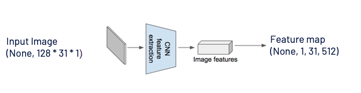
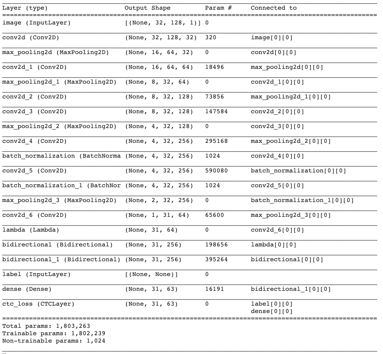
As seen from the above image, a grayscale image with width 128 and height 32 is sent through a series of convolutional & max-pooling layers. Layers are designed in such a manner that we obtain feature maps of the shape (None, 1, 31, 512) . “None” here is nothing but the batch size which could take any value.
(None, 1, 31, 512) can be easily reshaped to (None, 31, 512) , and 31 corresponds to the number of time steps, and 512 is nothing but the number of features at every time step. One can relate this to training any LSTM model with word embeddings like word2vec, Glove, fastText, and the input shape is usually like (batch_size, no_time_steps, word_embedding_dimension) .
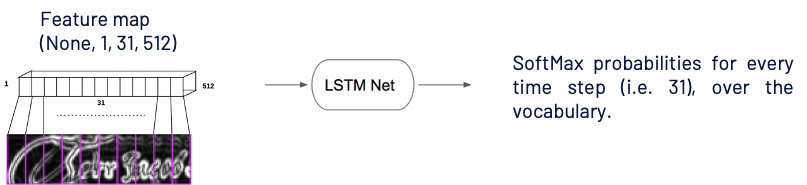
Later these feature maps are fed to the LSTM model, as shown above. You might be thinking now that LSTM models are known to work with sequential data and how feature maps are sequential!! Receptive fields play a significant role here 🙂 As one can see from the above image first value(first row, first column) in the feature map has visibility on the left part of the input image and last value(first row, last column) has visibility on the end part of the image, and yes this is sequential !!
From the LSTM model for every time step i.e., 31, we get a softmax probability over vocabulary. Now let us move on to the exciting part of the article on calculating the loss value for this architecture setup.
Calculating Loss
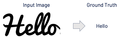
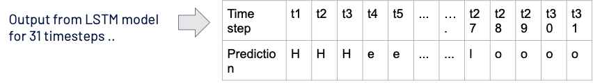
The length of ground truth is 5, which is not equal to the length of prediction i.e., 31.
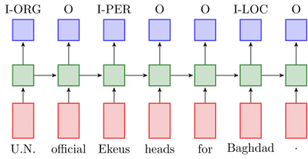
If we had ground truth for every time-step like the Named Entity Recognition(NER) task shown above, we could have used categorical cross-entropy as a loss. In the text recognition task, since we do not have ground truth for all the time steps i.e., 31, we cannot use cross-entropy loss.
Above mentioned scenario holds good for speech to text application as well. Audio signal and corresponding text are available as training data, and there is no mapping like the first character is spoken for “x” milliseconds or from “x1” to “x2” milliseconds character “z” is spoken.

Can we manually align each character to its location in the image /audio input?
The answer is yes. However, much manual effort is involved in creating training data. Forget about training a deep learning model that is always data hungry!
How do we calculate loss then? 🤔
CTC(Connectionist Temporal Classification) to the Rescue
With just the mapping of the image to text and not worrying about the alignment of each character to the input image’s location, one should be able to calculate the loss and train the network. Before moving on to calculating CTC loss, lets first understand the CTC decode operation.
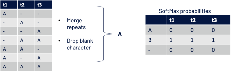
CTC Decode Operation

If we merge the repeats, we lose the repetitions, as shown in the above image. With just merging, we end up with a single letter “l,” which was supposed to be “ll.” So a special character called “blank character” is introduced to avoid this.

Now the decode operation consists of 2 steps: 1. Merge repeats 2. Remove blank characters. Now you can see “ll,” which is retained.
CTC loss
For simplicity lets say,
- the vocabulary is { A, B, – }
- we have predictions for 3-time steps from LSTM network (SoftMax probabilities over vocabulary at t1, t2, t3 )
Given that we use CTC decode operation discussed earlier, in which scenarios we can say output from the model is correct?
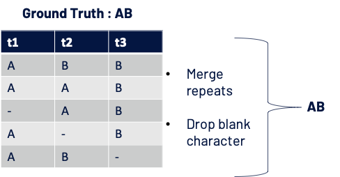
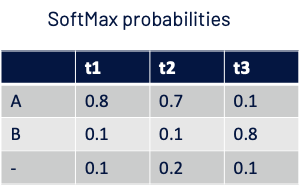
Let us say the Softmax probabilities for 3-time steps are as below:
Loss is calculated as – log(Probability of getting ground truth)
Probability of getting GT AB: = P(ABB) + P(AAB) + P(-AB) + P(A-B) + P(AB-)
Score for one path: AAB = (0.8 x 0.7 x 0.8) and similarly for other paths.
Why – log(Probability of getting ground truth) and why not (1 – Probability of getting ground truth) ? We will see below which one is better 🙂
CTC loss when there is a perfect match
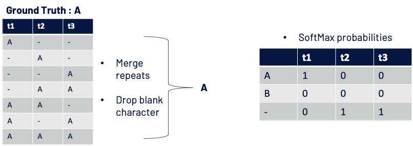
- Score for one path: A- – = (1 x 1 x 1) and similarly for other paths.
- Probability of getting ground truth A: = P(A–) + P(-A-) + P(–A) + P(-AA) + P(AA-) + P(A-A) + P(AAA) = 1 + 0 + 0 + 0 + 0 + 0 + 0
- Loss : – log( Probability of getting GT ) = – log( 1 ) = 0
CTC loss when there is perfect mismatch
- Score for one path: A – – = (0 x 0 x 0) and similarly for other paths.
- Probability of getting ground truth A: = P(A–) + P(-A-) + P(–A) + P(-AA) + P(AA-) + P(A-A) + P(AAA)
- Loss : – log( Probability of getting GT ) = tends to infinity
- If we had to use the loss as 1 – Probability of getting GT: a maximum penalty on the model for perfect mismatch would have been just 1.
As seen from the above examples, when there is a perfect match, both the loss functions yield the same value i.e., 0.
However, when there is a perfect mismatch if we use (1 – Probability of getting ground truth ), the penalty would be at max 1, but when we use – log(Probability of getting ground truth) the penalty tends to infinity!! So, now you know which is the better loss function !!
Code for CTC Loss
Let’s get to the coding part. One need not code all the math calculations covered above. We can use keras.backend.ctc_batch_cost for calculating the CTC loss and below is the code for the same where a custom CTC layer is defined which is used in both training and prediction parts.
class CTCLayer(layers.Layer):

    def __init__(self, name=None):

        super().__init__(name=name)
        self.loss_fn = keras.backend.ctc_batch_cost

    def call(self, y_true, y_pred):
        # Compute the training-time loss value and add it
        # to the layer using `self.add_loss()`.

        batch_len = tf.cast(tf.shape(y_true)[0], dtype="int64")
        input_length = tf.cast(tf.shape(y_pred)[1], dtype="int64")
        label_length = tf.cast(tf.shape(y_true)[1], dtype="int64")

        input_length = input_length * tf.ones(shape=(batch_len, 1), dtype="int64")
        label_length = label_length * tf.ones(shape=(batch_len, 1), dtype="int64")

        loss = self.loss_fn(y_true, y_pred, input_length, label_length)
        self.add_loss(loss)

        # At test time, just return the computed predictions
        return y_pred
Model Code and Architecture
def train(epochs):

    # input with shape of height=32 and width=128
    inputs = Input(shape=(32, 128, 1), name="image")

    labels = layers.Input(name="label", shape=(None,), dtype="float32")

    conv_1 = Conv2D(32, (3,3), activation = "selu", padding='same')(inputs)
    pool_1 = MaxPool2D(pool_size=(2, 2))(conv_1)

    conv_2 = Conv2D(64, (3,3), activation = "selu", padding='same')(pool_1)
    pool_2 = MaxPool2D(pool_size=(2, 2))(conv_2)

    conv_3 = Conv2D(128, (3,3), activation = "selu", padding='same')(pool_2)
    conv_4 = Conv2D(128, (3,3), activation = "selu", padding='same')(conv_3)

    pool_4 = MaxPool2D(pool_size=(2, 1))(conv_4)

    conv_5 = Conv2D(256, (3,3), activation = "selu", padding='same')(pool_4)

    # Batch normalization layer
    batch_norm_5 = BatchNormalization()(conv_5)

    conv_6 = Conv2D(256, (3,3), activation = "selu", padding='same')(batch_norm_5)
    batch_norm_6 = BatchNormalization()(conv_6)
    pool_6 = MaxPool2D(pool_size=(2, 1))(batch_norm_6)

    conv_7 = Conv2D(64, (2,2), activation = "selu")(pool_6)

    squeezed = Lambda(lambda x: K.squeeze(x, 1))(conv_7)

    # bidirectional LSTM layers with units=128
    blstm_1 = Bidirectional(CuDNNLSTM(128, return_sequences=True))(squeezed)
    blstm_2 = Bidirectional(CuDNNLSTM(128, return_sequences=True))(blstm_1)

    softmax_output = Dense(len(char_list) + 1, activation = 'softmax', name="dense")(blstm_2)

    output = CTCLayer(name="ctc_loss")(labels, softmax_output)


    optimizer = Adam(lr=0.001, beta_1=0.9, beta_2=0.999, clipnorm=1.0)

    #model to be used at training time
    model = Model(inputs=[inputs, labels], outputs=output)
    model.compile(optimizer = optimizer)

    print(model.summary())
    file_path = "C_LSTM_best.hdf5"

    checkpoint = ModelCheckpoint(filepath=file_path,
                                monitor='val_loss',
                                verbose=1,
                                save_best_only=True,
                                mode='min')

    callbacks_list = [checkpoint,
                      WandbCallback(monitor="val_loss",
                                    mode="min",
                                    log_weights=True),
                      PlotPredictions(frequency=1),
                      EarlyStopping(patience=3, verbose=1)]

    history = model.fit(train_dataset,
                        epochs = epochs,
                        validation_data=validation_dataset,
                        verbose = 1,
                        callbacks = callbacks_list,
                        shuffle=True)

    return model
Model Prediction on the Validation Data
Below is the GIF where you can see how the model learns to extract actual text from images starting from first to last epoch. Initially model predicts random text and after couple of epochs, one can see the predictions getting closer to the ground truth.
Currently, the model is trained using a subset of MJSynth open-source data. As you can see from the above image model is not able to accurately extract the text in there is cursive fonts or if the text is not clearly visible. One can include more such samples in the training data and train the model with those variations.
It is very difficult to manually prepare the dataset for these kinds of tasks. There are libraries like SynthText & Text Recognition Dataset Generator which help us to synthetically generate the data with varying fonts, font colors, background, etc .. Depending on the type of use case in hand one can decide whether to proceed with open-source datasets or to synthetically generate data for the same.
Full code for the CRNN-CTC model in Tensorflow is available here. Also, similar work was presented at Spark AI summit 2020, North America chapter.
