

This tutorial demonstrates how to preprocess audio files in the WAV format and build and train a basic automatic speech recognition (ASR) model for recognizing ten different words. You will use a portion of the Speech Commands dataset (Warden, 2018), which contains short (one-second or less) audio clips of commands, such as “down”, “go”, “left”, “no”, “right”, “stop”, “up” and “yes”.
This tutorial is originally hosted on the TensorFlow Tutorials page.
Real-world speech and audio recognition systems are complex. But, like image classification with the MNIST dataset, this tutorial should give you a basic understanding of the techniques involved.
Setup
Import necessary modules and dependencies. Note that you’ll be using seaborn for visualization in this tutorial.
import os
import pathlib

import matplotlib.pyplot as plt
import numpy as np
import seaborn as sns
import tensorflow as tf

from tensorflow.keras import layers
from tensorflow.keras import models
from IPython import display

# Set the seed value for experiment reproducibility.
seed = 42
tf.random.set_seed(seed)
np.random.seed(seed)
Import the Mini Speech Commands Dataset
To save time with data loading, you will be working with a smaller version of the Speech Commands dataset. The original dataset consists of over 105,000 audio files in the WAV (Waveform) audio file format of people saying 35 different words. This data was collected by Google and released under a CC BY license.
Download and extract the mini_speech_commands.zip file containing the smaller Speech Commands datasets with tf.keras.utils.get_file:
DATASET_PATH = 'data/mini_speech_commands'

data_dir = pathlib.Path(DATASET_PATH)
if not data_dir.exists():
  tf.keras.utils.get_file(
      'mini_speech_commands.zip',
      origin="http://storage.googleapis.com/download.tensorflow.org/data/mini_speech_commands.zip",
      extract=True,
      cache_dir='.', cache_subdir='data')
Downloading data from http://storage.googleapis.com/download.tensorflow.org/data/mini_speech_commands.zip
182083584/182082353 [==============================] - 6s 0us/step
182091776/182082353 [==============================] - 6s 0us/step
The dataset’s audio clips are stored in eight folders corresponding to each speech command: no, yes, down, go, left, up, right, and stop:
commands = np.array(tf.io.gfile.listdir(str(data_dir)))
commands = commands[commands != 'README.md']
print('Commands:', commands)
Commands: ['yes' 'go' 'left' 'right' 'up' 'down' 'stop' 'no']
Extract the audio clips into a list called filenames, and shuffle it:
filenames = tf.io.gfile.glob(str(data_dir) + '/*/*')
filenames = tf.random.shuffle(filenames)
num_samples = len(filenames)
print('Number of total examples:', num_samples)
print('Number of examples per label:',
      len(tf.io.gfile.listdir(str(data_dir/commands[0]))))
print('Example file tensor:', filenames[0])
Number of total examples: 8000
Number of examples per label: 1000
Example file tensor: tf.Tensor(b'data/mini_speech_commands/up/05739450_nohash_2.wav', shape=(), dtype=string)
Split filenames into training, validation and test sets using a 80:10:10 ratio, respectively:
train_files = filenames[:6400]
val_files = filenames[6400: 6400 + 800]
test_files = filenames[-800:]

print('Training set size', len(train_files))
print('Validation set size', len(val_files))
print('Test set size', len(test_files))
Training set size 6400
Validation set size 800
Test set size 800
Read the Audio Files and Their Labels
In this section you will preprocess the dataset, creating decoded tensors for the waveforms and the corresponding labels. Note that:
- Each WAV file contains time-series data with a set number of samples per second.
- Each sample represents the amplitude of the audio signal at that specific time.
- In a 16-bit system, like the WAV files in the mini Speech Commands dataset, the amplitude values range from -32,768 to 32,767.
- The sample rate for this dataset is 16kHz.
The shape of the tensor returned by tf.audio.decode_wav is [samples, channels], where channels is 1 for mono or 2 for stereo. The mini Speech Commands dataset only contains mono recordings.
test_file = tf.io.read_file(DATASET_PATH+'/down/0a9f9af7_nohash_0.wav')
test_audio, _ = tf.audio.decode_wav(contents=test_file)
test_audio.shape
TensorShape([13654, 1])
Now, let’s define a function that preprocesses the dataset’s raw WAV audio files into audio tensors:
def decode_audio(audio_binary):
  # Decode WAV-encoded audio files to `float32` tensors, normalized
  # to the [-1.0, 1.0] range. Return `float32` audio and a sample rate.
  audio, _ = tf.audio.decode_wav(contents=audio_binary)
  # Since all the data is single channel (mono), drop the `channels`
  # axis from the array.
  return tf.squeeze(audio, axis=-1)
Define a function that creates labels using the parent directories for each file:
- Split the file paths into
tf.RaggedTensors (tensors with ragged dimensions—with slices that may have different lengths).
def get_label(file_path):
  parts = tf.strings.split(
      input=file_path,
      sep=os.path.sep)
  # Note: You'll use indexing here instead of tuple unpacking to enable this
  # to work in a TensorFlow graph.
  return parts[-2]
Define another helper function—get_waveform_and_label—that puts it all together:
- The input is the WAV audio filename.
- The output is a tuple containing the audio and label tensors ready for supervised learning.
def get_waveform_and_label(file_path):
  label = get_label(file_path)
  audio_binary = tf.io.read_file(file_path)
  waveform = decode_audio(audio_binary)
  return waveform, label
Build the training set to extract the audio-label pairs:
- Create a
tf.data.DatasetwithDataset.from_tensor_slicesandDataset.map, usingget_waveform_and_labeldefined earlier.
You’ll build the validation and test sets using a similar procedure later on.
AUTOTUNE = tf.data.AUTOTUNE

files_ds = tf.data.Dataset.from_tensor_slices(train_files)

waveform_ds = files_ds.map(
    map_func=get_waveform_and_label,
    num_parallel_calls=AUTOTUNE)
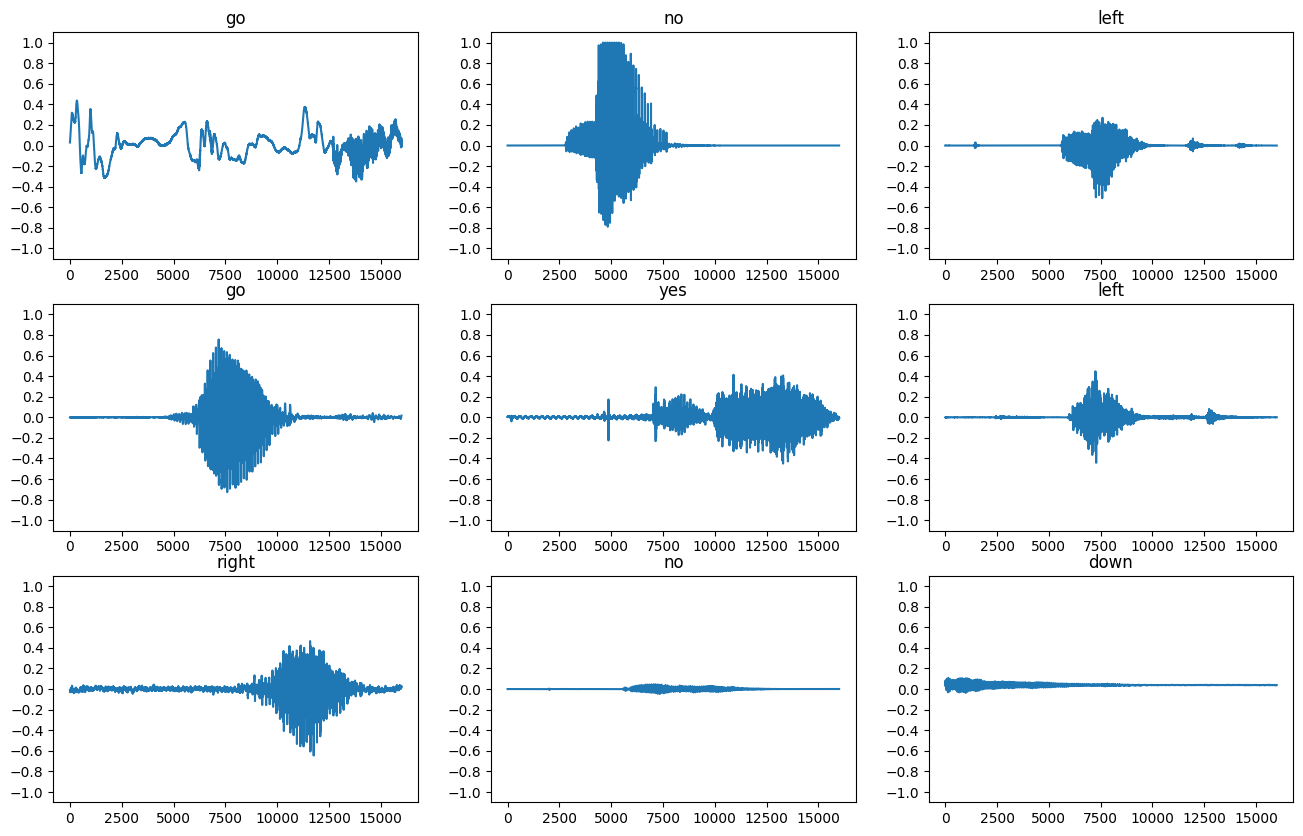
Let’s plot a few audio waveforms:
rows = 3
cols = 3
n = rows * cols
fig, axes = plt.subplots(rows, cols, figsize=(10, 12))

for i, (audio, label) in enumerate(waveform_ds.take(n)):
  r = i // cols
  c = i % cols
  ax = axes[r][c]
  ax.plot(audio.numpy())
  ax.set_yticks(np.arange(-1.2, 1.2, 0.2))
  label = label.numpy().decode('utf-8')
  ax.set_title(label)

plt.show()
Convert Waveforms to Spectrograms
The waveforms in the dataset are represented in the time domain. Next, you’ll transform the waveforms from the time-domain signals into the time-frequency-domain signals by computing the short-time Fourier transform (STFT) to convert the waveforms to as spectrograms, which show frequency changes over time and can be represented as 2D images. You will feed the spectrogram images into your neural network to train the model.
A Fourier transform (tf.signal.fft) converts a signal to its component frequencies, but loses all time information. In comparison, STFT (tf.signal.stft) splits the signal into windows of time and runs a Fourier transform on each window, preserving some time information, and returning a 2D tensor that you can run standard convolutions on.
Create a utility function for converting waveforms to spectrograms:
- The waveforms need to be of the same length, so that when you convert them to spectrograms, the results have similar dimensions. This can be done by simply zero-padding the audio clips that are shorter than one second (using
tf.zeros). - When calling
tf.signal.stft, choose theframe_lengthandframe_stepparameters such that the generated spectrogram “image” is almost square. For more information on the STFT parameters choice, refer to this Coursera video on audio signal processing and STFT. - The STFT produces an array of complex numbers representing magnitude and phase. However, in this tutorial you’ll only use the magnitude, which you can derive by applying
tf.abson the output oftf.signal.stft.
def get_spectrogram(waveform):
  # Zero-padding for an audio waveform with less than 16,000 samples.
  input_len = 16000
  waveform = waveform[:input_len]
  zero_padding = tf.zeros(
      [16000] - tf.shape(waveform),
      dtype=tf.float32)
  # Cast the waveform tensors' dtype to float32.
  waveform = tf.cast(waveform, dtype=tf.float32)
  # Concatenate the waveform with `zero_padding`, which ensures all audio
  # clips are of the same length.
  equal_length = tf.concat([waveform, zero_padding], 0)
  # Convert the waveform to a spectrogram via a STFT.
  spectrogram = tf.signal.stft(
      equal_length, frame_length=255, frame_step=128)
  # Obtain the magnitude of the STFT.
  spectrogram = tf.abs(spectrogram)
  # Add a `channels` dimension, so that the spectrogram can be used
  # as image-like input data with convolution layers (which expect
  # shape (`batch_size`, `height`, `width`, `channels`).
  spectrogram = spectrogram[..., tf.newaxis]
  return spectrogram
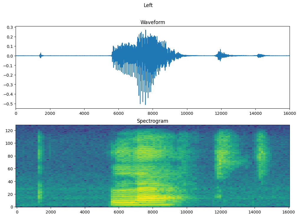
Next, start exploring the data. Print the shapes of one example’s tensorized waveform and the corresponding spectrogram, and play the original audio:
for waveform, label in waveform_ds.take(1):
  label = label.numpy().decode('utf-8')
  spectrogram = get_spectrogram(waveform)

print('Label:', label)
print('Waveform shape:', waveform.shape)
print('Spectrogram shape:', spectrogram.shape)
print('Audio playback')
display.display(display.Audio(waveform, rate=16000))
Label: up
Waveform shape: (11606,)
Spectrogram shape: (124, 129, 1)
Audio playback
Now, define a function for displaying a spectrogram:
def plot_spectrogram(spectrogram, ax):
  if len(spectrogram.shape) > 2:
    assert len(spectrogram.shape) == 3
    spectrogram = np.squeeze(spectrogram, axis=-1)
  # Convert the frequencies to log scale and transpose, so that the time is
  # represented on the x-axis (columns).
  # Add an epsilon to avoid taking a log of zero.
  log_spec = np.log(spectrogram.T + np.finfo(float).eps)
  height = log_spec.shape[0]
  width = log_spec.shape[1]
  X = np.linspace(0, np.size(spectrogram), num=width, dtype=int)
  Y = range(height)
  ax.pcolormesh(X, Y, log_spec)
Plot the example’s waveform over time and the corresponding spectrogram (frequencies over time):
fig, axes = plt.subplots(2, figsize=(12, 8))
timescale = np.arange(waveform.shape[0])
axes[0].plot(timescale, waveform.numpy())
axes[0].set_title('Waveform')
axes[0].set_xlim([0, 16000])

plot_spectrogram(spectrogram.numpy(), axes[1])
axes[1].set_title('Spectrogram')
plt.show()
Now, define a function that transforms the waveform dataset into spectrograms and their corresponding labels as integer IDs:
def get_spectrogram_and_label_id(audio, label):
  spectrogram = get_spectrogram(audio)
  label_id = tf.argmax(label == commands)
  return spectrogram, label_id
Map get_spectrogram_and_label_id across the dataset’s elements with Dataset.map:
spectrogram_ds = waveform_ds.map(
  map_func=get_spectrogram_and_label_id,
  num_parallel_calls=AUTOTUNE)
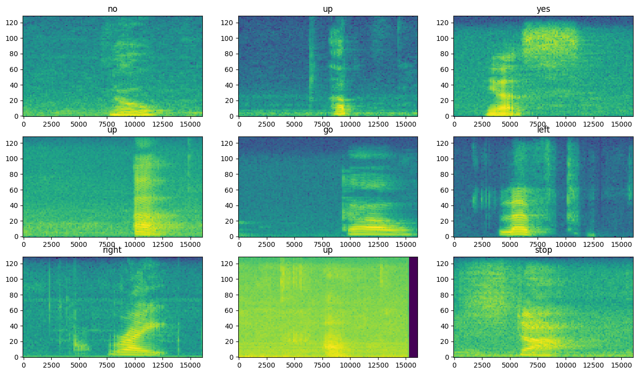
Examine the spectrograms for different examples of the dataset:
rows = 3
cols = 3
n = rows*cols
fig, axes = plt.subplots(rows, cols, figsize=(10, 10))

for i, (spectrogram, label_id) in enumerate(spectrogram_ds.take(n)):
  r = i // cols
  c = i % cols
  ax = axes[r][c]
  plot_spectrogram(spectrogram.numpy(), ax)
  ax.set_title(commands[label_id.numpy()])
  ax.axis('off')

plt.show()
Build and Train the Model
Repeat the training set preprocessing on the validation and test sets:
def preprocess_dataset(files):
  files_ds = tf.data.Dataset.from_tensor_slices(files)
  output_ds = files_ds.map(
      map_func=get_waveform_and_label,
      num_parallel_calls=AUTOTUNE)
  output_ds = output_ds.map(
      map_func=get_spectrogram_and_label_id,
      num_parallel_calls=AUTOTUNE)
  return output_ds
train_ds = spectrogram_ds
val_ds = preprocess_dataset(val_files)
test_ds = preprocess_dataset(test_files)
Batch the training and validation sets for model training:
batch_size = 64
train_ds = train_ds.batch(batch_size)
val_ds = val_ds.batch(batch_size)
Add Dataset.cache and Dataset.prefetch operations to reduce read latency while training the model:
train_ds = train_ds.cache().prefetch(AUTOTUNE)
val_ds = val_ds.cache().prefetch(AUTOTUNE)
For the model, you’ll use a simple convolutional neural network (CNN), since you have transformed the audio files into spectrogram images.
Your tf.keras.Sequential model will use the following Keras preprocessing layers:
For the Normalization layer, its adapt method would first need to be called on the training data in order to compute aggregate statistics (that is, the mean and the standard deviation).
for spectrogram, _ in spectrogram_ds.take(1):
  input_shape = spectrogram.shape
print('Input shape:', input_shape)
num_labels = len(commands)

# Instantiate the `tf.keras.layers.Normalization` layer.
norm_layer = layers.Normalization()
# Fit the state of the layer to the spectrograms
# with `Normalization.adapt`.
norm_layer.adapt(data=spectrogram_ds.map(map_func=lambda spec, label: spec))

model = models.Sequential([
    layers.Input(shape=input_shape),
    # Downsample the input.
    layers.Resizing(32, 32),
    # Normalize.
    norm_layer,
    layers.Conv2D(32, 3, activation='relu'),
    layers.Conv2D(64, 3, activation='relu'),
    layers.MaxPooling2D(),
    layers.Dropout(0.25),
    layers.Flatten(),
    layers.Dense(128, activation='relu'),
    layers.Dropout(0.5),
    layers.Dense(num_labels),
])

model.summary()
Input shape: (124, 129, 1)
Model: "sequential"
_________________________________________________________________
 Layer (type)                Output Shape              Param #
=================================================================
 resizing (Resizing)         (None, 32, 32, 1)         0

 normalization (Normalizatio  (None, 32, 32, 1)        3
 n)

 conv2d (Conv2D)             (None, 30, 30, 32)        320

 conv2d_1 (Conv2D)           (None, 28, 28, 64)        18496

 max_pooling2d (MaxPooling2D  (None, 14, 14, 64)       0
 )

 dropout (Dropout)           (None, 14, 14, 64)        0

 flatten (Flatten)           (None, 12544)             0

 dense (Dense)               (None, 128)               1605760

 dropout_1 (Dropout)         (None, 128)               0

 dense_1 (Dense)             (None, 8)                 1032

=================================================================
Total params: 1,625,611
Trainable params: 1,625,608
Non-trainable params: 3
_________________________________________________________________
Configure the Keras model with the Adam optimizer and the cross-entropy loss:
model.compile(
    optimizer=tf.keras.optimizers.Adam(),
    loss=tf.keras.losses.SparseCategoricalCrossentropy(from_logits=True),
    metrics=['accuracy'],
)
Train the model over 10 epochs for demonstration purposes:
EPOCHS = 10
history = model.fit(
    train_ds,
    validation_data=val_ds,
    epochs=EPOCHS,
    callbacks=tf.keras.callbacks.EarlyStopping(verbose=1, patience=2),
)
Epoch 1/10
100/100 [==============================] - 13s 40ms/step - loss: 1.7404 - accuracy: 0.3823 - val_loss: 1.3372 - val_accuracy: 0.5550
Epoch 2/10
100/100 [==============================] - 0s 4ms/step - loss: 1.1776 - accuracy: 0.5903 - val_loss: 0.9747 - val_accuracy: 0.6600
Epoch 3/10
100/100 [==============================] - 0s 4ms/step - loss: 0.9027 - accuracy: 0.6778 - val_loss: 0.8096 - val_accuracy: 0.7150
Epoch 4/10
100/100 [==============================] - 0s 4ms/step - loss: 0.7647 - accuracy: 0.7316 - val_loss: 0.7325 - val_accuracy: 0.7625
Epoch 5/10
100/100 [==============================] - 0s 4ms/step - loss: 0.6492 - accuracy: 0.7658 - val_loss: 0.6697 - val_accuracy: 0.7688
Epoch 6/10
100/100 [==============================] - 0s 5ms/step - loss: 0.5796 - accuracy: 0.7937 - val_loss: 0.6108 - val_accuracy: 0.7875
Epoch 7/10
100/100 [==============================] - 0s 4ms/step - loss: 0.5261 - accuracy: 0.8117 - val_loss: 0.5708 - val_accuracy: 0.8087
Epoch 8/10
100/100 [==============================] - 0s 4ms/step - loss: 0.4747 - accuracy: 0.8267 - val_loss: 0.5429 - val_accuracy: 0.8163
Epoch 9/10
100/100 [==============================] - 0s 4ms/step - loss: 0.4427 - accuracy: 0.8428 - val_loss: 0.5379 - val_accuracy: 0.8175
Epoch 10/10
100/100 [==============================] - 0s 4ms/step - loss: 0.3927 - accuracy: 0.8637 - val_loss: 0.5320 - val_accuracy: 0.8213
Let’s plot the training and validation loss curves to check how your model has improved during training:
metrics = history.history
plt.plot(history.epoch, metrics['loss'], metrics['val_loss'])
plt.legend(['loss', 'val_loss'])
plt.show()

Evaluate the Model Performance
Run the model on the test set and check the model’s performance:
test_audio = []
test_labels = []

for audio, label in test_ds:
  test_audio.append(audio.numpy())
  test_labels.append(label.numpy())

test_audio = np.array(test_audio)
test_labels = np.array(test_labels)
y_pred = np.argmax(model.predict(test_audio), axis=1)
y_true = test_labels

test_acc = sum(y_pred == y_true) / len(y_true)
print(f'Test set accuracy: {test_acc:.0%}')
Test set accuracy: 84%
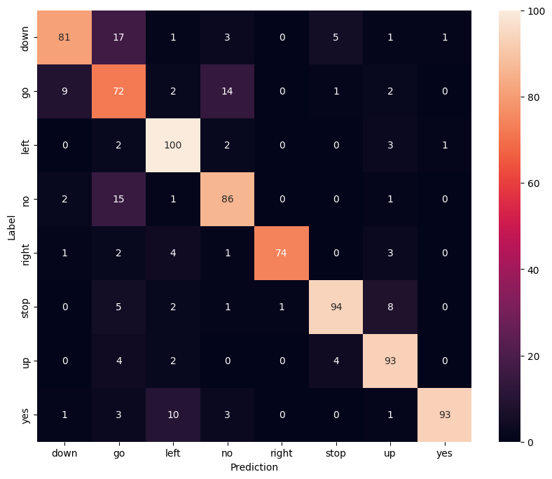
Display a confusion matrix
Use a confusion matrix to check how well the model did classifying each of the commands in the test set:
confusion_mtx = tf.math.confusion_matrix(y_true, y_pred)
plt.figure(figsize=(10, 8))
sns.heatmap(confusion_mtx,
            xticklabels=commands,
            yticklabels=commands,
            annot=True, fmt='g')
plt.xlabel('Prediction')
plt.ylabel('Label')
plt.show()
Run Inference on an Audio File
Finally, verify the model’s prediction output using an input audio file of someone saying “no”. How well does your model perform?
sample_file = data_dir/'no/01bb6a2a_nohash_0.wav'

sample_ds = preprocess_dataset([str(sample_file)])

for spectrogram, label in sample_ds.batch(1):
  prediction = model(spectrogram)
  plt.bar(commands, tf.nn.softmax(prediction[0]))
  plt.title(f'Predictions for "{commands[label[0]]}"')
  plt.show()
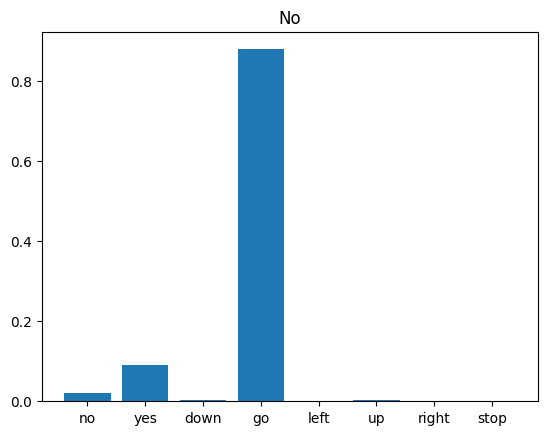
As the output suggests, your model should have recognized the audio command as “no”.
Next steps
This tutorial demonstrated how to carry out simple audio classification/automatic speech recognition using a convolutional neural network with TensorFlow and Python. To learn more, consider the following resources:
- The Sound classification with YAMNet tutorial shows how to use transfer learning for audio classification.
- The notebooks from Kaggle’s TensorFlow speech recognition challenge.
- The TensorFlow.js – Audio recognition using transfer learning codelab teaches how to build your own interactive web app for audio classification.
- A tutorial on deep learning for music information retrieval (Choi et al., 2017) on arXiv.
- TensorFlow also has additional support for audio data preparation and augmentation to help with your own audio-based projects.
- Consider using the librosa library—a Python package for music and audio analysis.
